
Title: IMAGE COMPRESSION BASED ON PREDICTION CODING
Authors: Rajesh Mandale, Akshay Mhetre & Rahul Nikam , Researchers, E&TC Department
Guide: Prof. Dr.V.K.Bairagi, Associate Professor, E&TC Department
Institute: AISSMS’s Institute of Information Technology, University of Pune, Pune.
ABSTRACT
Image processing plays an important role in multimedia. It helps to reduce file size for hardware storage requirement and fast transition time. Prediction coding technique is a lossless image compression method. The prediction coding is the most simple for encoding and decoding. It also helps in low computational complexity and overheads. Predictive coding can be made superior with the help of compression ratio and time algorithm. This paper summarizes the basic prediction coding algorithms and their improvements by using various techniques. On the basis of the analysis, a new algorithm is proposed. Aim of this paper is to make a superior lossless predictive coding technique for image compression on the basis of following – 1. Compression ratio 2. Time
Keywords- Image compression, Prediction coding, Lossless image, Compression ratio
I. INTRODUCTION
Processing of digital images involve procedures that are usually expressed in algorithmic form due to which most image processing functions are implemented in software. It deals with manipulation of images. The image signal may be either digital or analog. There are a wide range of image processing operations. In addition to photography, the field of digital imaging has created a whole range of new applications and tools that were previously impossible. Face recognition software, medical image processing and remote sensing are all possible due to the development of digital image processing. Specialized computer programs are used to enhance and correct images. Everyday a huge amount of information is stored, processed, and transmitted. Because much of this information is in the form of pictures and graphs in nature, the storage and communications requirements are very much. Image compression refers to the problem of reducing the amount of data requirements to represent a digital image.
The term data compression means the process of reducing the amount of data required to represent a given quantity of information. Various amount of data can be used to represent the same information.Data might contain elements that provide no relevant information is called data redundancy.
There are two types of image compression lossy compression and lossless compression. Lossless compression involves compressing data which, when decompressed, will be an exact replica of the original data. This is the case when binary data such as executables, documents etc. are compressed. They need to be exactly reproduced when decompressed. But in case of lossy image compression, when decompressed, will not an exact replica of the original image. For lossless image compression we are using predictive coding. Predictive coding means there will be transmission of difference between the current pixel and the previous pixel.
II. IMAGE COMPRESSION OVERVIEW
Image processing techniques were first developed in 1960 through the combined work of various scientists and academics. The main focus of their work was to develop medical imaging, character recognition and create high quality images at the microscopic level. During this era, equipment and processing costs were relatively high.
The financial problems had a serious impact on the depth and breadth of technology development that could be done. There are three major benefits to digital image processing, the consistent high quality of the image, the low cost of processing and the ability to manipulate all aspects of the process are all great benefits. As long as computer processing speed continues to increase and the cost of memory continues to drop, the field of image processing will grow.
There are two types in compression such as lossy compression and lossless compression. Lossy compression is a data encoding method that compresses data by discarding some of it. The procedure aims to reduce the amount of data that needs to be transmitted by a computer. Typically, a significant amount of data can be discarded before the result is sufficiently degraded to be noticed by the user. Lossless compression involves compressing data which, when decompressed, will be an exact replica of the original data. This is the case when binary data such as executables, documents etc. are compressed. They need to be exactly reproduced when decompressed.
There are different types of lossless compression which are –
1] Dictionary coding
2] Entropy coding
3] Predictive Coding.
There are some major disadvantages of the first two types, so we are focusing on predictive coding. The three types of predictive coding are – Median Edge Detector (MED), Gradient Adjusted Predictor (GAP) and Gradient Edge Detector (GED).
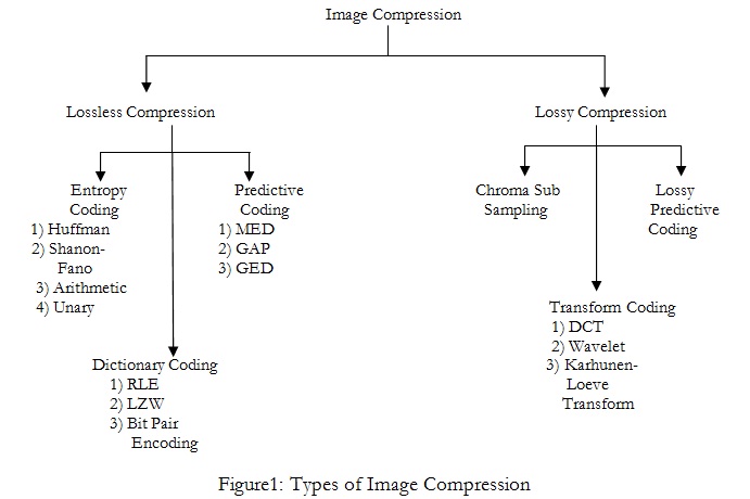
III. IMAGE COMPRESSION CLASSIFICATION
These are different types of image compression. In Lossless compression there is no loss of data and hence lossless image compression is preferred. There are few disadvantages of Dictionary and Entropy coding. The disadvantage of dictionary codes is that these codes are usually efficient only for long files. Short files can actually result in the transmission (or storage) of more bits. And in Entropy coding, major problem is that if there are some codes which have the same ending as the beginning as some other codes, we can’t differentiate between codes. And Predictive coding is much simpler technique.
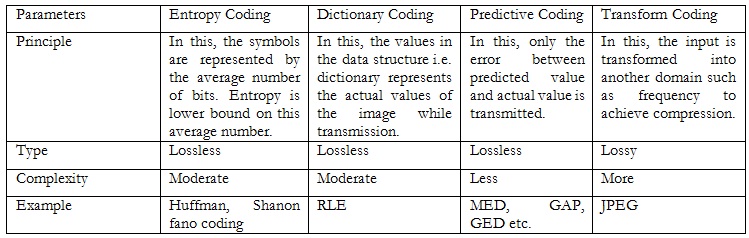
Difference between different types of coding
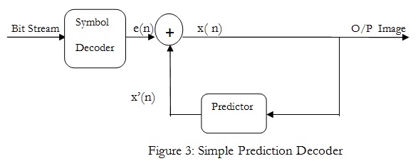
IV. BLOCK DIAGRAM
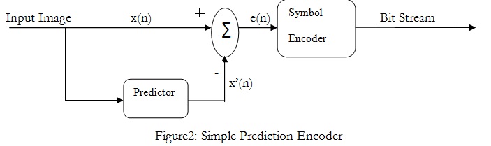
For most images, there are redundancies among adjacent pixel values; that is, adjacent pixels are highly correlated. Thus, a current pixel can be predicted reasonably well based on a neighborhood of pixels. The prediction error, which is obtained by subtracting the prediction from the original pixel, has smaller entropy than the original pixels. Hence, the prediction error can be encoded with fewer bits. In the predictive coding, the correlation between adjacent pixels is removed and the remaining values are encoded.
V. METHODS IMPLEMENTED
1) Median edge detector (MED):-
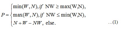
Median Edge Detection (MED) belongs to the group of switching predictors that select one of the three optimal sub predictors depending on whether it found the vertical edge horizontal edge, or smooth region [5]. In fact, MED predictor selects the median value between three possibilities W, N and W + N – NW (common labels are chosen after sides of the world), and the optimal combination of simplicity and efficiency. The prediction is based on [8] –
2) Gradient adjusted predictor (GAP):-
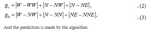
Gradient Adjusted Predictor (GAP) is based on gradient estimation around the current pixel [7]. Gradient estimation is estimated by the context of current pixel, which in combination with predefined thresholds gives final prediction [7]. GAP distinguishes three types of edges, strong, simple and a soft edge, and is characterized by high flexibility to different regions. Gradient estimation is by [7]-
Here we have proposed a solution that takes advantage of the MED and GAP predictors i.e. simplicity of the median predictor and advantages of gradient estimation in GAP predictor. As MED predictor, chooses between the context of vertical edges, horizontal edges and smooth regions. Selection is done by simple estimation of horizontal and vertical gradient and one threshold.
3) Gradient Estimation Detector (GED):-
The number of contextual pixel is also a compromise between the MED and GAP predictors, and in contrast to the GAP predictor, which has three predefined threshold, the proposed predictor is based on one threshold. Gradient estimation is based on the equation; predictor is based on edge detection, so we adopt the name of the Gradient Edge Detection (GED). GED local gradient estimation is done using following equations:
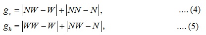
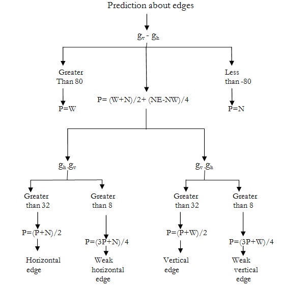
local gradient estimation is followed by a simple predictor. The prediction is done using the algorithm [8]:
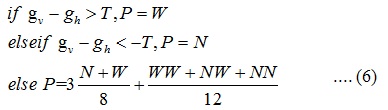
Where T is the threshold, which can be predefined or may be based on the context. Second is GED2 predictor, which is slightly different from the first one in the case when smooth region is detected. For the estimation of local gradient, is also used above equation. Complicated and inefficient equation is replaced by same equation that uses MED predictor in the case of smooth region. Therefore, GED2 prediction is made by following equation:
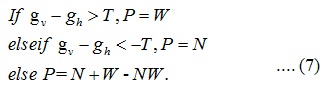
GED2 predictor is a simple combination of gradient and median predictors. Estimation of local gradient and a threshold is used to decide which of the three sub predictors is optimal, i.e. is the pixel in context of horizontal edge, vertical edge or smooth region.
4) Blending predictor:-
The idea of blending predictors is nothing but forming a set of sub predictors. Its concept is to make a new technique which takes the advantages of other technique and discarding the disadvantages. This predictor is used to generate a new superior technique. The works of G. Deng show high efficiency of the blending predictor method. Using blending technique new algorithm can be proposed which is not only time efficient, but has also excellent data compression performance. We have analyzed non-linear predictors that are based on contextual switching between constant predictors.
The simplest version is three-context median filter MED, GAP and GED. Each of these proposals is suitable for encoding without delays, as they do not require introductory computation. There is no rule that among m constant predictors selection of n sub predictors yielding the lowest entropy values leads to the best results in the blending prediction method. But use of Blending Predictor increases complexity in the algorithm and gives best result.
5) Compressive Sensing:- Compressive sensing was introduced by Donoho in 2006.Compressive Sensing is the new theory which is different from traditional sampling. Then the question may arise that what’s wrong with the old nyquist sampling theory? The problem in traditional sampling is that huge information is acquired in this sampling, but most of it is waste.
DIFFERENCE BETWEEN TRADITIONAL SAMPLING AND COMPRESSIVE SENSING
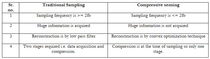
An image is given as input to the Compressive sensing block. In this few samples having more information are acquired and simultaneously compression takes place. These few samples transmitted from transmitter through the medium and received at the receiver. Reconstruction of original image is done using convex optimization.
VI. TABLES
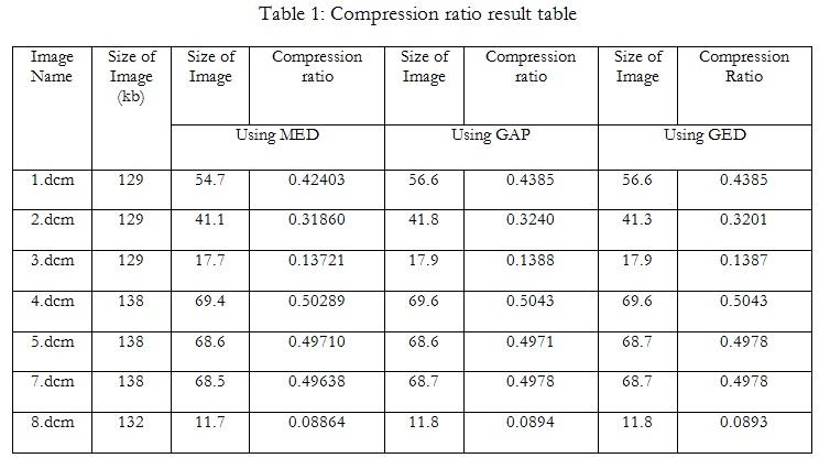
1) This table shows compression ratio of an image using three lossless predictive coding technique i.e. MED, GAP, GED. 2)Out of three methods, using MED technique compressed image size is less than GAP and GED. For example consider 3.dcm image, its compressed image size is less i.e. 17.7kb compared with other two techniques.
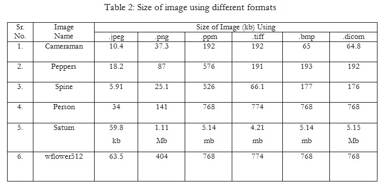
1) This table shows size of image using different image formats i.e. .jpeg, .png, .ppm, .tiff, .bmp, .dicom. 2) From this table it is concluded that the size of image using JPEG format is less than other formats while size of image using BMP format is more but quality is also more.
WHAT WE ARE GOING TO DO?
The objective of this paper is to reduce irrelevance and redundancy of the image data in order to be able to store or transmit data in an efficient form. The goal is to take advantage of spatial redundancy & coding redundancy in image, the idea is to use previous pixel value to predict the next pixel value. To make a superior lossless predictive coding technique for image compression on the basis of following – 1. Compression ratio 2. Time
VII. APPLICATIONS
1) ECG (Electro Cardio Graph)
2) Camera: in all digital camera, images stored in JPEG format. Since it compress all images at most till today. Instead of that by using predictive coding algorithm we can compress more.
3) Medical Imaging: MRI, CT scan images: In all medical equipments captured image have to be stored in image .This algorithm can compress all dicom image file.
VIII. CONCLUSION
We have studied prediction based compression algorithms such as MED, GAP, GED, and it is concluded that these algorithms are lossless. The compression ratios obtained after operation varies w.r.t. image and data. It is concluded that the single algorithm is not efficient in all the cases, hence this concluded that there is requirement of new algorithm which will take into consideration the image data. This may be achieved using combination of various basic algorithms. While combining this algorithm one thing one must consider that the complexity algorithm should not increase beyond certain limit unlike in blending predictor.
REFERENCES
[1] Pan Z. et al,2010, “A Lossless Compression Algorithm for SAR Amplitude Imagery Base on Modified Quadtree Coding of Bit Plane”, IEEE geoscience and remote sensing letters, Vol.7, No.4, pp. 723-726.
[2] Liu Z., Qian Y., Yang L., Bo Y., and Li H., “ A improved lossless image compression algorithm LOCO R”, International Conference on Computer Design and Applications (ICCDA), Vol. 1, 2010, pp. 328-331.
[3] Hu Y. C. and Su B. H., 2008, “ Accelerated K-Means clustering algorithm for color image quantization”,
Imaging science journal, The, Vol. 56, No. 1, pp. 29-40
[4]Bankman I.N.,2009: “Handbook of Medical Image Processing and Analysis, Elsevier”, London
[5] Chen X.., 2008, “Lossless compression for space imagery in a dynamically reconfigurable architecture,” in Proceedings of International Workshop on Applied Reconfigurable Computing, LNCS 4943, pp. 336-341. [6] Andriani S., Calvagno G., Erseghe T., Mian G. A., Durigon M., Rinaldo R., Knee M., Walland P., and Koppetz M., 2004, “Comparison of lossy to lossless compression techniques for digital cinema,” in Proceedings of International Conference on Image Processing, Vol. 1, pp. 513-516.
[7] Memon N. and Wu X., 1997: “Recent Developments in Context-based Predictive Techniques for Lossless Image Compression”, The Computer Journal, Vol. 40, No. 2/3, pp. 127 – 136.
[8] Wienberger M.J., Seroussi G. and Sapiro G., March/April 1996: LOCO-I: “A Low Complexity, Context-based, Lossless Image Compression Algorithm,” Conference on Data Compression, Snowbird, UT, USA, pp.140 – 149.
[9] Nandedkar V., Kumar S.V.B. and Mukhopadhyay S., March 2005: “Lossless Volumetric Medical Image Compression with Progressive Multiplanar Reformatting using 3DDPCM”, National Conference on Image Processing, Bangalore, India.
[10] Wallace G. K., Apr.1991 “The jpeg still picture compression standard,” Communications of the ACM”.
[11] Shiroma, J. T. , 2006. “An introduction to DICOM. Veterinary Medicine”, 19-20. Retrieved from http://0search.proquest.com.alpha2.latrobe.edu.au/docview/195482647?accountid=12001
[12] Pennebaker W. B. & Mitchell J. L. , 1993 ,“JPEG Still Image Data Compression Standard ”, New York: Van Nostrand Reinhold. ISBN 0-442-01272-1.
[13] Seemann T. and Tisher P., “Generalized locally adaptive DPCM,” Technical Report
CS97/301, Department of Computer Sciencek, Monash University, pp. 1-15.
[14] Wu X and Memon N., May 1996: CALIC – “A Context based Adaptive Lossless Image Codec, IEEE International Conference on Acoustics, Speech, and Signal Processing”, Atlanta, GA, USA, Vol. 4, pp. 1890 – 1893