Title: Agent Modeling for the Simulation of a Simple Smart Micro grid
Authors: Ms.S.Swathi & Mr.Sundaraiah Nayini
Organisation: Malla Reddy Engineering College for Women
Abstract– The smart grid is a highly complex system that is being formed from the traditional power grid, adding new and sophisticated communication and control devices. This will enable integrating new elements for distributed power generation and also achieving an increasingly automated operation so for actions of the utilities as for customers. In order to model such systems a bottom-up method is followed, using only a few basic elements which are structured into two layers: a physical layer for the electrical power transmission, and one logical layer for element communication. A simple case study is presented to analyze the possibilities of simulation. It shows a micro grid model with dynamic load management and an integrated approach that can process both electrical and communication flows.
Keywords:- Power grid, smart grid, renewable energy systems, energy saving, smart meter, micro grid modeling, complex systems, agent-based modeling, demand side management, smart grid simulation, load flow, load shedding
INTRODUCTION
In the last years energy systems are moving away from a centralized and hierarchical structure, under strict control of the electricity supply companies, towards a new system where distributed actors influence the energy supply. Production is no longer limited to large energy providers, as small decentralized producers in the form of distributed generation (DG) enter the network and are able to inject energy at much lower voltage levels than before. This paradigm shift involves new challenges for the modeling and simulation of energy systems for which decentralized models are needed. Among the presented in a review in [1], there are for example several commercial tools used in power engineering, such as Euro stag or PSS/E. Further, a number of non-proprietary tools exist, such as several toolboxes based on Mat lab/Semolina, for example Manpower or PSAT. Since some years the term smart grid has become widespread in the energy sector. The introduction of smart grids involves a change from manual operations towards an intelligent, ICT based and controlled network. These changes will especially affect the distribution grid [2], and in this way, micro grids.
A number of models have been developed to analyze and understand the behavior of micro grids. Some of them focused on decentralized control strategies, usually using Mat lab/Semolina and similar classic tools, are of special interest [3, 4, 5]. Particularly relevant is the work on demand side management, using virtual powers plants [6] and on multivalent platforms [7]. And also worth mention as significant the recently extended idea, discussed in some conferences [8] and accepted very well in some countries, of using micro grids as building blocks of the future smart grid [9].
Here we recall that traditional methods used for analysis of electrical networks are based on static power flow calculations [10]. But these methods are not suitable for computing the system response to special events (such as power changes in generators fed by renewable energies, sudden connection and disconnection of loads and sources, or even when the network structure changes after a disaster occurs), because in these cases the values of the variables have to be updated in a short time, as they are used for the network control or simulation, and therefore a new “steady” state computation is required each time one of such special event occurs, which is not efficient at all. Trying to give a solution to this problem the authors designed a decentralized power flow algorithm for this kind of models (see below). This method provides a more flexible and dynamic way than traditional methods and is able to cope with sudden changes and disasters.
Modeling the smart grid In [11], the complexity for modeling smart grids was identified. A first smart grid model was developed, which represents the system on the physical layer, by integrating a distributed load flow algorithm. The model was tested by running different simulations, letting interact a wind generation unit, a photovoltaic panel, a battery, two loads and a diesel generator. By modeling the individual elements as agents, a modular and flexible approach was used, where the agents can be programmed to have different behaviors such as the charging and discharging times for the battery system, or the integration of variable wind speeds by adding a wind speed simulator module which directly interacts with the turbines. On the logical layer, a first approach was made. This approach is extended in the current work by adding real-time communications to the simulation, which represent one of the main features of the logical layer. Because of their scarce resources, micro grids need a flexible demand side [13], so introducing communication is essential as it allows performing monitoring, control [14] and demand side management, among others. As some specific aspects of the author’s work in this area were presented in some conferences [11, 15, 16, 11, 17], in a rather informal manner, here we intend to offer a more understandable and reproducible description of them, by using some elements from the ODD protocol [18].
Modeling the smart grid:-
In [11], the complexity for modeling smart grids was identified. A first smart grid model was developed, which represents the system on the physical layer, by integrating a distributed load flow algorithm. The model was tested by running different simulations, letting interact a wind generation unit, a photovoltaic panel, a battery, two loads and a diesel generator. By modeling the individual elements as agents, a modular and flexible approach was used, where the agents can be programmed to have different behaviors such as the charging and discharging times for the battery system, or the integration of variable wind speeds by adding a wind speed simulator module which directly interacts with the turbines. On the logical layer, a first approach was made. This approach is extended in the current work by adding real-time communications to the simulation, which represent one of the main features of the logical layer. Because of their scarce resources, micro grids need a flexible demand side [13], so introducing communication is essential as it allows performing monitoring, control [14] and demand side management, among others. As some specific aspects of the author’s work in this area were presented in some conferences [11, 15, 16, 11, 17], in a rather informal manner, here we intend to offer a more understandable and reproducible description of them, by using some elements from the ODD protocol [18].
OVERVIEW
An agent-based approach was chosen for modelling a simple microgrid, trying to represent a minimalistic smart grid (or smart-microgrid). The implementation was done in the multi-paradigm modelling environment AnyLogic.
Purpose:-
The main aim is to demonstrate the feasibility and convenience of the agent based methods in that small instance, and further be able to use it as a building block [8] in other more complex power networks, and even to grow it to other more capable multiple layered structures, able to deal with multicarrier energy networks. The model is intended to be very flexible and, although its actual size was chosen to be very small, in order to simplify explanations and demonstrations, it may be easily adapted to any other given microgrid structure. This shall allow for practically any virtual experiment for control and management schemes, some of which, still under development, are required for a sustainable operation of microgrids within the energy system [14].
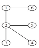
Figure 1: Graph of the model electrical network
A very first and simplified model of a load management is proposed, using communicating smart meters. The model focuses on the system view, which rather than representing the load management mechanism in detail, aims to represent the microgrid as a whole in order to observe the effects at that level. The model shows the importance of a logical layer in the smart grid.
Structure – state variables and scales:-
The model structure is inspired on power flow analysis [10]. In this context an electrical network is represented by a weighted graph G = (V, E) where V is a set of n vertices and E ∈ {V × V} is the set of edges in the network. Figure 1 shows a graph with six vertices, representing the simple electric network of the model. Vertices are also called buses by electrical engineers and represent electrical power generators and loads, and edges, also called lines, represent electrical power transmission lines. Physically, an electrical network represents a circuit where the electricity is flowing from each node to some other. The approach the authors proposed in [11] is to split the network node in two parts, in order to obtain a two layer structure, composed of a logical layer and a physical layer. An agent is assigned to each node – so there are also n agents – who acting at the two layers are able to perform their respective tasks: power flow calculations at the physical layer, communications tasks at the logical layer, and also the implied inter-layer actions. The very simple example showed in Figure 2, with six agents, has been chosen for instantiate the model. Note the number of vertices is the same, n = 6, for both layers but the edges are different: while at the logical layer edges represent communication channels so, at the physical layer they represent electric lines. These figures also shows the vertex numbers and their type in the physical layer: Slack, Control and Load, also named respectively Reference, PV and PQ buses, referring to the known real data pair at the two last.
Process overview and scheduling:-
At the lowest level, like a daemon, the AnyLogic simulation engine is conducting the most basic rhythms for the launched model, using a well defined, scheduled pattern of time and event steps. During each time step, the model clock is advanced, the discrete state of the model remains unchanged, active equations, if any, are being solved numerically, the variables are changed correspondingly and also awaited change events are tested for occurrence. During each event step, no model time elapses, the actions of states, transitions, events, ports, etc. corresponding to this event are executed, the discrete state of the model may change, some scheduled events may be deleted, and the new events may be scheduled in the AnyLogic Engine event queue. At any simulation time, the user can view the event queue of the AnyLogic simulation engine to view what is happening there and even to make some changes to the event processing (see The Big Book of AnyLogic [19]). This amazing process is one of the main virtues of the program since it frees the user from the complicated task of treating events, greatly facilitating the implementation of discrete event models. At the highest level, the Main Class allows the user for instantiate all the other classes corresponding to submodels, agents creation and replication, main variables definition, model initialisation, and also to create the user interface and some her complementary variables. This class is associated with the so called Main Window, through which the user define the main parameters and variables and instantiate the classes. A specially important instance here is the Environment one (whose class can be found in the AnyLogic libraries), where the agents “live”, because it is usually used to define the basic rules for agent behaviour. Agent interactions are created at two layers (see Figure 2. At the physical layer they are given by electrical circuit laws (Ohm and Kirchhoff’s law, etc.) translated to computational power flow algorithm rules. At the logical layer, interactions represent internal and external events, and they are implemented as agent messages in the model. The agents are also able to carry out other grid tasks such as power flow control, generation unit dispatch, load dispatch and shedding, grid connection and disconnection, etc.
A.Process at the logical layer:- In broad outline, the “Control Unit”, is located in the substation at the bus 1. This place is also called Point of Common Coupling (PCC) because it is where the microgrid can be coupled/decoupled from the main grid. Here there is a special ICT equipment that monitors the power and sends the message “Peak” or “OffPeak” to the consumer SmartMeters. To monitor the power, first the control unit calibrates itself, i.e. obtains the average power (P¯) the first day, to be used after as a threshold to detecting peaks. Then it check if there is a peak power (power P in the substation is greater than bP¯), or not (P in the substation is less than aP¯), where a = 0, 8 and b = 1.2 were chosen. While none of these conditions is met, the system stays in the previous state (hysteresis). The process is described in the flowchart in Figure 3. The consumers, as described in the flowchart in Figure 4, analyse the content of the message. If the state is “Peak” then they reduce their load by the energy save factor esf which is set equal to 0.4 (40%) in the model. If it is “OffPeak”, the value of this factor is set to 1.
B. Process at the physical layer:- The main task that agents perform during simulation is the decentralised power flow algorithm specially designed by the authors for this kind of models [11]. This method provides a more flexible and dynamic way than traditional methods and is able to cope with sudden changes and disasters. At each environment’s time step, the algorithm updates the voltage (magnitude and angle) of each node as an harmonic function of all connected nodes. It was extended with a smart meter and a local load management system which are able to communicate with the point of common coupling (PCC) of the microgrid. The PCC is able to sense the state of the grid and communicate with the consumers in order to request them to control their loads.
C. Power Flow calculus:-
The Ohm law of a network, in matrix form, is I = YV

Figure 2: The two layers for the microgrid example
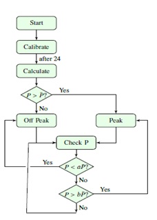
Figure 3: Process at the Control Unit
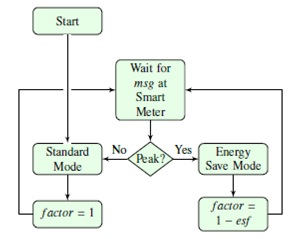
Figure 4: Process at consumer agents
If V is given (and also if I is given), equation 1 represents a linear system of equations, whose solution can be obtained using standard linear algebra methods or relaxations methods. But that is not the case because, for typical electrical network problems, three different kind of buses exist, each with different specified variables, and then a non-linear system of 2n equations on 2n real unknowns results. Let us review the matter briefly. Each bus in a power system can be classified in one of three types:
- Slack bus: voltage magnitude and phase are speci- fied – active and reactive powers are unknown
- PV bus: voltage magnitude and active power are specified – phase angle and reactive power are un-known
- PQ bus: active and reactive power are specified – voltage magnitude and phase are unknown
DESIGN CONCEPTS
As mentioned before, two kind of interactions occur in the model. At the physical layer these interactions are intended to perform the electrical behaviour of the network, by implementing a power flow algorithm, and therefore they do a completely deterministic, imposed, process. But at the logical layer, interactions are as result of agent communications and so agent behaviours can became rather complex, because they use specific rules which possibly depend of a number of environmental, most of them stochastic, variables. This can arise to emergent phenomena such as agent synchronisation [21], usually not desirable, and other effects. Probably, the best goodness the model can offer is prediction. Answer to questions like “what happens if . . . ?” can be useful in a lot of situations, especially in designing communication, control and operation systems, where a number of procedures and devices should be tested in simulation before the actual implementation is performed.
DETAILS
Submodels :-
- Elements of the microgrid:-
The microgrid model aims to include most of the aspects of future smart grids: distributed generation, renewable energy sources and communication flows are represented. The model consists of the following elements:
- 1 Point of Common Coupling (PCC) – bus 1
- 1 Diesel generator – bus 2
- 2 Load (consumers) – buses 3 and 4
- 1 Wind turbine – bus 5 • 1 Photovoltaic panel, linked to
- 1 Battery storage system – bus 6
The load model includes the necessary elements to allow its management through a smart meter device.
- Load modeling:-
A typical averaged curve which represents the active power of households was assumed. To add some randomness to the behaviour, the curve is overlaid with white Gaussian noise. On the physical layer, a consumer is modelled as a PQ bus, with the reactive demand set to zero, (it can be negligible in residential uses).
- The smart meter as an inter-layer device:-
Devices acting on both layers are represented in a dual way. An agent on the physical layer represents a node of the electrical grid and its behaviour is de- fined by the physical equations concerning power flow. Each physical agent is mapped to a logical agent, which handles the communications and all other interactions which are not on the load flow layer. Each logical agent is linked to its physical agent trhough a pointer, and is able to access and manage values like the active power. The implementation of a first inter-layer device is shown by a basic smart meter, which collects consumer information and sends it to an aggregator. It was embedded into the logical agent of the consumer. This smart meter collects information about the consumption from the physical agent and is capable to send it to the PCC. Further, the smart meter is capable to receive load management requests from the PCC, i.e. a signal which will tell the consumer to reduce its consumption at given times.
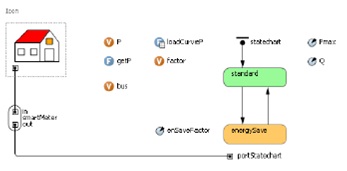
Figure 5: Logical layer model of a load (consumer) with an embedded smart meter and load management system
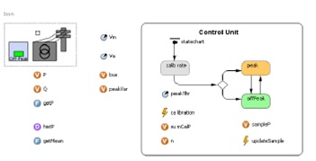
Figure 6: PCC / Substation logical layer model with control unit
The smart meter is embedded in the consumer agent (see Figure 5) and is able to act on the load. The actuation on the load is represented intentionally in a very simple way, as there exist many different techniques for load management (e.g. it can be performed in an automatised way, due to the customer’s behaviour, caused by incentives, etc.). In this case, a generic reduction of the load, independently on how it is achieved, is modelled, which is sufficient for the current model.
- The PCC and the control unit:-
On the physical layer, the PCC is modelled as the slack bus, i.e. the complex voltage value is fixed (to the magnitude of the base voltage value of the p.u. system), and the voltage angle set to zero. On the logical layer, the PCC is able to gather the consumption of all the consumers of the microgrid through its communication with the smart meters. The PCC integrates the control unit, which is able to take decisions based on two inputs: a) The aggregated or individual load values of the consumers, which were gathered through the logical layer interconnection b) The physical layer values such as the P and Q values at the PCC bus The latter gives information about the balancing of the grid and whether there is over-production or overconsumption. The consumer data allows to know how much the net consumption (without batteries or production devices) is. The control unit selects the peak periods by regarding the average power of the previous day and fixing the threshold (this process is called calibration). When the active power at the PCC is greater than this threshold, a peak period is assumed (see Figure 3). In the case of a peak period, the control unit will begin sending messages over the logical layer to the consumers when the the threshold is surpassed. Different strategies can be tested by observing a) and b) separately or a combination of them. In this example case, only b) is observed. In this case, the message will be a load reduction request to the consumers, which will reduce their load by a defined factor, in this case 40%. A feedback loop in the system is created, which is indirectly controlling household loads. The active load is monitored by the PCC control unit, managed through messages over the logical layer. This has an effect on the loads on the physical layer which through the integrated power flow on this layer will influence the the active load at the PCC bus. Additionally, other units of the system, mainly producers, which have a partially random behaviour (modelled by white Gaussian noise), will perturb the system. To avoid oscillation, a small hysteresis element is included at the peak detection (with a = 0.8 and b = 1.2), see section 2.3.1. This load management allows better optimising the energy system. From the economic point of view, adapting the load by e.g. reducing peaks avoids the use of expensive peak power plants. By giving the user incentives by dynamic tariffs that reflect the higher costs to the consumer it is possible to reduce the loads. Being able to manage the load of a microgrid allows to use it as a flexible module of the electrical system in the sense of a virtual power plant, which supports and improves the overall efficiency of the power system
SIMULATION RESULTS
The simulation main window appears in Figure 7. It shows the model structure, including the logical layer and the physical layer, with the bus index and type, the voltage magnitude and angle, and the active and reactive powers, at each bus. Note that the connections in both layers are the same as in Figure 2. The figure also shows the icons of the main instances in the model: the environment, the agents and the Excel file where the data to build the example are written. The PCC includes a control unit, which surveys the active power at the PCC. This allows to determine the production-demand balance of the microgrid. When the power is over a certain threshold, the control unit sends a signal (which could be imagined as a tariff signal) to the customers, which indicates a peak period. We assume that the consumer reacts to this signal by reducing the consumption by a certain amount (during the peak period, a more expensive tariff can be imagined, so either the user or an automated system will lower the load). In the simulation, the following production and load behaviours are assumed:
- The diesel generator produces a continuous power of 5 kW
- The PV panel produces power according to a sinusoidal profile (sunny day) with some random noise and a peak power of 5 kW
- The battery charges during the day (11-17h) and discharges in the evening (20-23h) at +/- 5 kW
- The wind generator is coupled to a wind speed simulator and produces varying powers up to 10 kW
- The consumers are modelled using a standard pro- file, where consumer1 has a peak load of 15 kW and consumer2 of 18 kW.
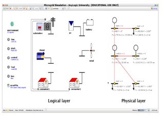
Figure 7: Simulation main window
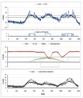
Figure 8: Active powers of the simulated microgrid case study
The energy reduction factor is 40% for each. This makes a total installed generation capacity is 20 kW (which is only partially available due to the fluctuating renewables). The total load can reach up to 33 kW (but is usually much below this value). Additionally, +/- 5 kW of the battery are available, which can operate as load or pseudo-generation. The simulation results of one day are shown in Figure 8. The active powers, which are decisive for the load management, are shown. A limit (which is obtained by the control unit at the PCC automatically based on the average power from the previous day) which defines peak and off-peak periods can be seen around 4 kW. Positive powers at the PCC describe an unbalance in the microgrid towards under-generation (less than consumed is generated in the microgrid). The higher these values, the more energy has to be imported from the external grid to the microgrid. The peak periods are de- fined as the values above 4 kW and shown in the second chart separately. The third chart represents the generation units and their respective generated active powers. Wind generation is relatively stable, except during the afternoon and evening. Solar power is depending on radiation, so a quasi-sinusoidial curve. The battery was scheduled to charge and discharge at fixed times (see above). In the bottom chart, the loads of consumer2 are shown. Here we can see the effect of the signal sent by the PCC control unit during peak times to the consumer. In order to evaluate the impact of the load management system, a load curve for consumer2 is shown in light gray which represents a day without reductions. We can clearly see that the loads are mainly reduced during peak times. Peak times are evaluated in real time at the control unit, so sending peak signals has an immediate, but effect on the power of the PCC. This explains that some oscillations can occur (for example the short peaks between minutes 1080-1200).
CONCLUSION
The given example model implements a very simple load management algorithm, to show feasibility of the simulation model. The communication mechanism between the PCC and the consumers allows monitoring powers and send signals to the consumers, which leads to a load management. The combination of several approaches allows the creation of models that might abstract some details from the single unit models, but all in all create a much more realistic representation at the system level. The inclusion of some communication among the devices is fundamental here. A combined approach seems reasonable and advantageous. Classical tools hardly allow the implementation of dynamic interaction and message passing among the individual devices. The agent-based approach, which is combined with a classical load flow treats the simulation from a different point of view. The case study shows the interest of being able to reproduce both effects on the power grid and the communication network, and observe the complex system behavior as a whole. Future works include the improvement of the load model, which is very simple for the moment, as well as the load management algorithm, in order to reduce oscillations and other not desired effects. Measurements are being carried out with tests on real loads, to validate these models.
FURTHER CONSIDERATIONS
There are two parallel networks, which are however closely related to each other. The logical layer represents the information transfer, based on ICT [23]. The electrical flows and phenomena can be influenced by decisions obtained with the information of the communication network. Therefore, communication and interlayer devices are needed. Because Any Logic gives facilities to easily implement communications between agents, the user only have to instantiate and use them, by calling the appropriate methods. As in the example presented Any logic connectors were used, then at the simulation steps, messages pass automatically from an agent to other connected agent. Note that this facility enables the user to model communications without using any actual device. Also the smart meter object modeled is independent of technology. This allows the user to model without any concern about devices that will be eventually used, so the election of the actual technologies can be postponed, allowing the future use of any technology. It is specially interesting in situations where some of implicated devices are not yet ready, or even they do not exist, becoming a very helpful tool for them.
REFERENCES
[1] B. Valor, S. Heifer, Software for analysis of integration possibility of renewable energy units into electrical networks, in: The 5th International Conference Electric Power Quality and Supply Reliability, Proceedings Tallinn University of Technology pp 173-177., Vim’s, Estonia, 2006.
[2] F. Jejuna, S. Bolas, The evolution of distribution, Power and Energy Magazine, IEEE 7 (2009) 63–68. 1540-7977.
[3] M. Radanovich, T. C. Green, High-quality power generation through distributed control of a power park micro grid, Industrial Electronics, IEEE Transactions on 53 (2006) 1471–1482.
[4] N. Hatziargyriou, A. Dimes, A. Tsikalakis, Centralized and decentralized control of micro grids, International Journal of Distributed Energy Resources 1 (2005) 197–212.
[5] C. Suita, D. W. Mania, M. G. Samos, Distributed intelligent energy management system for a single-phase high-frequency ac micro grid, Industrial Electronics, IEEE Transactions on 54 (2007) 97–109.
[6] P. Polanski, F. Kudzu, A. A. Said, Z. Kai, Modeling domestic housing loads for demand response, in: Industrial Electronics, 2008. IECON 2008. 34th Annual Conference of IEEE, 2008, pp. 2742–2747.
[7] S. Thesis, V. Vasyutynskyy, K. Kabitzsch, Software agents in industry: A customized framework in theory and praxis, Industrial Informatics, IEEE Transactions on 5 (2009) 147–156.
[8] N. Hatziargyriou, Microgrids: Building blocks of the smart grid, Panel, 2012. URL: Available: http://www.ieee-isgt-2012.eu/events/ micro grids-building-blocks-of-the-smart-grid/.
[9] M. Erol-Kantarci, B. Kantars, H. Mouth, Cost-aware smart micro grid network design for a sustainable smart grid, in: GLOBECOM Workshops (GC Wisps), 2011 IEEE, 2011, pp. 1178 –1182.
[10] A. Bergen, V. Vital, Power System Analysis, Prentice Hall, New Jersey, 2000.
[11] E. Kermes, P. Viejo, J. M. Gonzalez de Duran, O. Bar ambones, A complex systems modeling approach for decentralized simulation of electrical micro grids, in: 15th IEEE International Conference on Engineering of Complex Computer Systems, Oxford, 2010.
[12] F. Milano, Power system analysis toolbox, 2009. URL: www.power.uwaterloo.ca/∼Milano/psat.htm.
[13] P. Polanski, D. Dietrich, Demand side management: Demand response, intelligent energy systems, and smart loads, Industrial Informatics, IEEE Transactions on 7 (2011) 381–388.
[14] O. Alsayegh, S. Alhajraf, H. Albusairi, Grid-connected renewable energy source systems: Challenges and proposed management schemes, Energy Conversion and Management 51 (2010) 1690–1693.
To download the above paper in PDF format Click on below Link: